Geometric methods for conical surfaces and intersecting spherical caps

Introduction

This vignette explores the geometric methods for computing solid angles of conical surfaces, polyhedral cones, and intersecting spherical caps, based on the work of Mazonka (2012) [1]. These methods provide intuitive, geometrically motivated approaches that complement the algebraic series methods. We cover right circular cones with the classic solid angle formula; polyhedral cones using the Van Oosterom & Strackee formula; cone segments representing partial circular cones; solid angle of intersection regions for intersecting cones; and interactive visualization with 3D plotly graphics.

library(SolidAngleR)

# Check if visualization packages are available
has_plotly <- requireNamespace("plotly", quietly = TRUE)
has_viridis <- requireNamespace("viridisLite", quietly = TRUE)

if (!has_plotly || !has_viridis) {
  message("Note: plotly and/or viridisLite not available. ",
          "Some visualizations will be skipped.")
}

Right circular cones

Mathematical formula

A right circular cone with apex at the origin and half-apex angle \(\theta\) has solid angle:

\[\Omega(\theta) = 2\pi(1 - \cos\theta)\]

For the normalized measure (fraction of sphere):

\[\omega(\theta) = \frac{\Omega(\theta)}{4\pi} = \frac{1 - \cos\theta}{2}\]

Properties

In the small angle limit, \(\Omega \approx \pi\theta^2\) for \(\theta \ll 1\); for a hemisphere, \(\theta = \pi/2 \Rightarrow \Omega = 2\pi\); and for the full sphere, \(\theta = \pi \Rightarrow \Omega = 4\pi\).

Examples

# Test various apex angles (exclude endpoints to avoid edge cases)
theta_values <- seq(0.01, pi - 0.01, length.out = 20)

# Vectorized computation (solid_angle_cone accepts vectors)
omega_values <- solid_angle_cone(theta_values)

# Convert to degrees for readability
theta_degrees <- theta_values * 180 / pi

# Show select values
select_indices <- c(1, 5, 10, 15, 20)
cone_table <- data.frame(
  theta_deg = theta_degrees[select_indices],
  omega_normalized = omega_values[select_indices],
  percent_sphere = omega_values[select_indices] * 100
)
knitr::kable(
  cone_table,
  digits = c(1, 6, 2),
  col.names = c("theta (deg)", "omega (normalized)", "percent of sphere")
)

theta (deg)	omega (normalized)	percent of sphere
0.6	0.000025	0.00
38.2	0.107214	10.72
85.3	0.458973	45.90
132.4	0.836894	83.69
179.4	0.999975	100.00


library(ggplot2)
df_circ <- data.frame(theta_deg = theta_degrees, omega = omega_values)

ggplot(df_circ, aes(theta_deg, omega)) +
  geom_vline(xintercept = c(45, 90, 135), colour = "grey85",
             linetype = 2, linewidth = 0.4) +
  geom_hline(yintercept = c(0.25, 0.5, 0.75), colour = "grey85",
             linetype = 2, linewidth = 0.4) +
  geom_line(colour = "#3B528B", linewidth = 0.9) +
  geom_point(data = data.frame(theta_deg = 90, omega = 0.5),
             colour = "#E15759", size = 2.6) +
  ylim(0, 1) +
  labs(title    = "Circular cone solid angle vs. apex angle",
       subtitle = expression(paste("Mazonka closed form ", omega == (1 - cos(theta)) / 2)),
       x = expression(paste("apex angle ", theta, " (degrees)")),
       y = expression(paste("normalized solid angle ", omega)),
       caption = "Source: solid_angle_cone(). Red dot at theta = 90 marks the hemisphere.") +
  theme_minimal(base_size = 11) +
  theme(plot.caption = element_text(color = "grey40", size = 8, hjust = 0))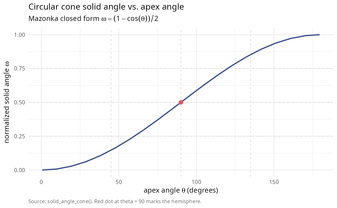

Small angle approximation

For small angles, we verify the approximation \(\Omega \approx \pi\theta^2\):

# Test small angles
theta_small <- c(0.01, 0.05, 0.1, 0.2, 0.3)
omega_exact <- sapply(theta_small, solid_angle_cone) * 4 * pi  # Convert to steradians
omega_approx <- pi * theta_small^2

small_angle_table <- data.frame(
  theta_rad = theta_small,
  omega_exact_sr = omega_exact,
  omega_approx_sr = omega_approx,
  rel_error = abs(omega_exact - omega_approx) / omega_exact
)
knitr::kable(
  small_angle_table,
  digits = c(3, 6, 6, 2),
  col.names = c("theta (rad)", "exact (sr)", "approx (sr)", "rel. error")
)

theta (rad)	exact (sr)	approx (sr)	rel. error
0.01	0.000314	0.000314	0.00
0.05	0.007852	0.007854	0.00
0.10	0.031390	0.031416	0.00
0.20	0.125245	0.125664	0.00
0.30	0.280629	0.282743	0.01

Polyhedral cones (Van Oosterom & Strackee formula)

Mathematical formula

For a polyhedral cone defined by vertices \(\mathbf{v}_1, \mathbf{v}_2, \ldots, \mathbf{v}_n\) on the unit sphere, the Van Oosterom & Strackee (1983) [2] formula provides:

\[\Omega = \sum_{\text{faces}} \left( \sum_{\text{angles}} - (n-2)\pi \right)\]

For a triangular face with vertices \(\mathbf{a}, \mathbf{b}, \mathbf{c}\):

\[\Omega = \arctan\left(\frac{|\mathbf{a} \cdot (\mathbf{b} \times \mathbf{c})|}{1 + \mathbf{a} \cdot \mathbf{b} + \mathbf{b} \cdot \mathbf{c} + \mathbf{c} \cdot \mathbf{a}}\right)\]

Examples

# Example 1: Simple triangle on unit sphere
# Create three points on the unit sphere forming a triangle
v1 <- c(1, 0, 0)
v2 <- c(0, 1, 0)
v3 <- c(1, 1, 0) / sqrt(2)  # 45 degrees from both v1 and v2

vertices_simple <- cbind(v1, v2, v3)

omega_simple <- solid_angle_polyhedral(vertices_simple)

# Example 2: Right triangle (orthant)
v1 <- c(1, 0, 0)
v2 <- c(0, 1, 0)
v3 <- c(0, 0, 1)

vertices_right <- cbind(v1, v2, v3)

omega_right <- solid_angle_polyhedral(vertices_right)

# Example 3: Narrow triangle
v1 <- c(1, 0, 0)
v2 <- c(0.99, 0.1, 0) / sqrt(0.99^2 + 0.1^2)
v3 <- c(0.99, -0.1, 0) / sqrt(0.99^2 + 0.1^2)

vertices_narrow <- cbind(v1, v2, v3)

omega_narrow <- solid_angle_polyhedral(vertices_narrow)

polyhedral_table <- data.frame(
  case = c("Simple triangle", "Right triangle (octant)", "Narrow triangle"),
  omega_sr = c(omega_simple, omega_right, omega_narrow) * 4 * pi,
  omega_normalized = c(omega_simple, omega_right, omega_narrow),
  percent_sphere = c(omega_simple, omega_right, omega_narrow) * 100,
  error_vs_octant = c(NA, abs(omega_right - 0.125), NA)
)
knitr::kable(
  polyhedral_table,
  digits = c(NA, 6, 6, 2, 2),
  col.names = c("case", "omega (sr)", "omega (normalized)",
                "percent of sphere", "error vs. 1/8")
)

Cone segments

A cone segment in Mazonka (2012) is the portion of a right circular cone cut by a plane. The plane is specified by the angle \(\gamma\) between the cone axis and the plane normal (equivalently, the segment is the intersection of the cone with a hemisphere whose boundary plane has that normal).

Mathematical formula

For an acute cone and a valid intersection, define:

\[ \phi = \arccos\!\left(\frac{\cos\gamma}{\tan\theta}\right), \qquad \beta = \arccos\!\left(\frac{\sin\gamma}{\sin\theta}\right). \]

Then the segment solid angle (steradians) is:

\[\Omega_{\text{segment}} = 2\left(\phi - \cos\theta \cdot \beta\right).\]

We report the normalized value \(\omega = \Omega/(4\pi)\). Special cases:

\(\gamma = 0\) returns the full cone.
If \(\gamma > \pi/2 + \theta\), the plane misses the cone and \(\Omega = 0\).
For \(\gamma > \pi/2\), symmetry gives an equivalent angle \(\gamma_{\mathrm{eff}} = \pi - \gamma\).

The package implementation uses the analytic expression when valid and falls back to numerical integration near boundary cases.

Examples

# Cone segments with various parameters
test_segments <- data.frame(
  theta_deg = c(30, 45, 60, 60),
  gamma_deg = c(0, 30, 60, 80)
)

test_segments$theta_rad <- test_segments$theta_deg * pi / 180
test_segments$gamma_rad <- test_segments$gamma_deg * pi / 180

segment_results <- data.frame(
  theta_deg = test_segments$theta_deg,
  gamma_deg = test_segments$gamma_deg,
  omega_sr = NA_real_,
  omega_normalized = NA_real_
)

for (i in 1:nrow(test_segments)) {
  theta <- test_segments$theta_rad[i]
  gamma <- test_segments$gamma_rad[i]
  omega <- solid_angle_cone_segment(theta, gamma)
  segment_results$omega_sr[i] <- omega * 4 * pi
  segment_results$omega_normalized[i] <- omega
}

knitr::kable(
  segment_results,
  digits = c(0, 0, 4, 6),
  col.names = c("theta (deg)", "gamma (deg)", "omega (sr)", "omega (normalized)")
)

theta (deg)	gamma (deg)	omega (sr)	omega (normalized)
30	0	0.8418	0.066987
45	30	1.8403	0.146447
60	60	2.5559	0.203393
60	80	2.9407	0.234017

Intersecting cones

One of the most interesting applications is computing the solid angle of the region where two circular cones intersect.

Mathematical setup

Two circular cones with: - Apex angles: \(\theta_1, \theta_2\) - Separation angle between axes: \(\alpha\)

The intersection region has solid angle that depends on all three parameters. In SolidAngleR, solid_angle_intersecting_cones() uses a robust spherical-cap overlap integral by default, with an optional analytic method for acute cones. Special cases (no overlap, containment, two hemispheres, and opposite axes) are handled explicitly. A Monte Carlo fallback is available for cross-checking or difficult geometries.

Computation

# Test various intersection scenarios
test_intersections <- list(
  list(name = "Equal cones, small separation",
       theta1 = pi/6, theta2 = pi/6, alpha = pi/12),
  list(name = "Equal cones, medium separation",
       theta1 = pi/4, theta2 = pi/4, alpha = pi/3),
  list(name = "Different cones, moderate separation",
       theta1 = pi/3, theta2 = pi/4, alpha = pi/6),
  list(name = "Wide cones, close together",
       theta1 = pi/2.5, theta2 = pi/3, alpha = pi/8),
  list(name = "Two hemispheres, 90°",
       theta1 = pi/2, theta2 = pi/2, alpha = pi/2)
)
intersection_table <- data.frame(
  case = character(),
  theta1_deg = numeric(),
  theta2_deg = numeric(),
  alpha_deg = numeric(),
  omega_normalized = numeric(),
  percent_sphere = numeric(),
  stringsAsFactors = FALSE
)

for (test in test_intersections) {
  omega_int <- solid_angle_intersecting_cones(
    test$theta1,
    test$theta2,
    test$alpha
  )
  intersection_table <- rbind(intersection_table, data.frame(
    case = test$name,
    theta1_deg = test$theta1 * 180 / pi,
    theta2_deg = test$theta2 * 180 / pi,
    alpha_deg = test$alpha * 180 / pi,
    omega_normalized = omega_int,
    percent_sphere = omega_int * 100
  ))
}

knitr::kable(
  intersection_table,
  digits = c(NA, 1, 1, 1, 6, 2),
  col.names = c("case", "theta1 (deg)", "theta2 (deg)", "alpha (deg)",
                "omega (normalized)", "percent of sphere")
)

case	theta1 (deg)	theta2 (deg)	alpha (deg)	omega (normalized)	percent of sphere
Equal cones, small separation	30	30	15.0	0.046335	4.63
Equal cones, medium separation	45	45	60.0	0.034978	3.50
Different cones, moderate separation	60	45	30.0	0.124173	12.42
Wide cones, close together	72	60	22.5	0.232482	23.25
Two hemispheres, 90°	90	90	90.0	0.250000	25.00

Interactive 3D visualization

The package provides the plotIntersectingCones() function for interactive visualization of intersecting cones using plotly.

Basic visualization

# Default parameters
fig1 <- plotIntersectingCones(
  theta1 = pi/6,  # 30-degree first cone
  theta2 = pi/4,  # 45-degree second cone
  phi = pi/3,     # 60-degree separation
  cone_opacity = 0.2,
  show_rays = FALSE
)

fig1

Varying cone parameters

Let’s explore how the intersection region changes with different parameters:

Case 1: Small cones, close together

fig_case1 <- plotIntersectingCones(
  theta1 = pi/8,   # Narrow first cone
  theta2 = pi/8,   # Narrow second cone
  phi = pi/6,      # Close separation
  color_palette = "plasma",
  cone_opacity = 0.25,
  show_rays = TRUE
)

fig_case1

Case 2: Wide cones, moderate separation

fig_case2 <- plotIntersectingCones(
  theta1 = pi/3,   # 60-degree cone
  theta2 = pi/2.5, # ~72-degree cone
  phi = pi/4,      # 45-degree separation
  color_palette = "viridis",
  cone_opacity = 0.15,
  show_rays = FALSE
)

fig_case2

Parameter exploration

Let’s systematically explore how solid angle varies with separation:

# Fix cone angles, vary separation
theta1 <- pi/4
theta2 <- pi/3
phi_values <- seq(0, pi/2, length.out = 20)

omega_intersection <- sapply(phi_values, function(phi) {
  solid_angle_intersecting_cones(theta1, theta2, phi)
})

library(ggplot2)
omega1 <- solid_angle_cone(theta1)
omega2 <- solid_angle_cone(theta2)

df_int <- data.frame(phi_deg = phi_values * 180 / pi,
                     omega   = omega_intersection)

ggplot(df_int, aes(phi_deg, omega)) +
  geom_hline(yintercept = omega1, colour = "#E15759",
             linetype = 2, linewidth = 0.5) +
  geom_hline(yintercept = omega2, colour = "#3B528B",
             linetype = 2, linewidth = 0.5) +
  geom_line(colour = "#1F1F1F", linewidth = 0.9) +
  labs(title    = bquote("Intersection vs. separation (" *
                            theta[1] * "=" *
                            .(sprintf("%.0f", theta1 * 180 / pi)) * degree * ", " *
                            theta[2] * "=" *
                            .(sprintf("%.0f", theta2 * 180 / pi)) * degree * ")"),
       subtitle = "Mazonka closed-form intersection of two circular cones",
       x = expression(paste("separation angle ", phi, " (degrees)")),
       y = "intersection solid angle (normalized)",
       caption = "Source: solid_angle_intersecting_cones(). Red and blue dashed lines: individual cone areas.") +
  theme_minimal(base_size = 11) +
  theme(plot.caption = element_text(color = "grey40", size = 8, hjust = 0))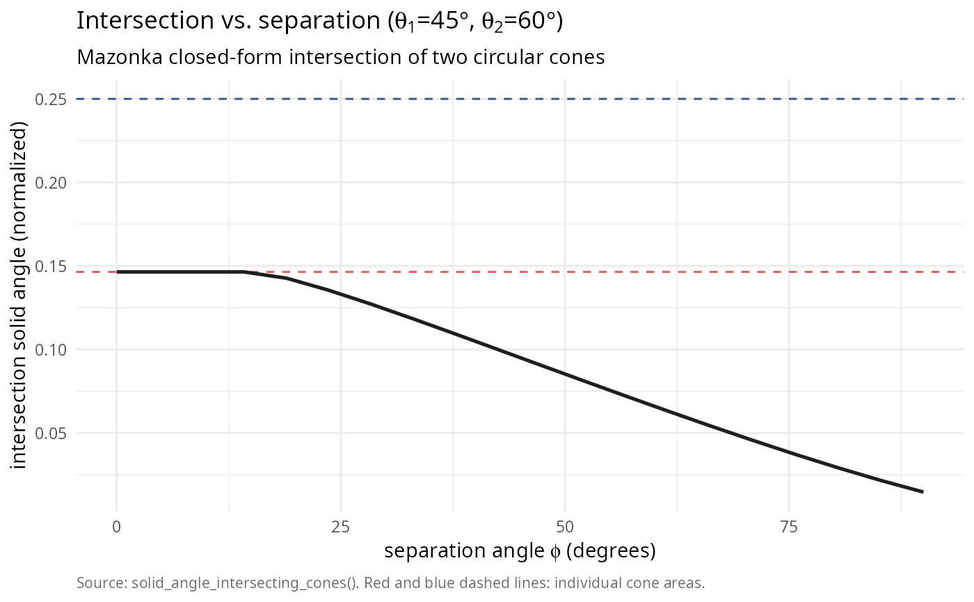

Comparison with algebraic methods

For cones that can be expressed both geometrically and as polyhedral cones, we can compare the different computational methods:

# Create a cone that can be computed both ways
theta <- pi/3
n_sides <- 8  # Approximate circular cone with octagonal cone

# Create octagonal cone vertices
angles <- seq(0, 2*pi, length.out = n_sides + 1)[-(n_sides + 1)]
radius <- sin(theta)
height <- cos(theta)

vertices_octagon <- rbind(
  radius * cos(angles),
  radius * sin(angles),
  rep(height, n_sides)
)

# Normalize to unit sphere
vertices_octagon <- apply(vertices_octagon, 2, function(v) v / sqrt(sum(v^2)))

# Method 1: Geometric (circular cone)
omega_geometric <- solid_angle_cone(theta)

# Method 2: Polyhedral (average over faces)
omega_polyhedral_faces <- numeric(n_sides)
for (i in 1:n_sides) {
  j <- ifelse(i == n_sides, 1, i + 1)
  face <- cbind(c(0, 0, 1), vertices_octagon[, i], vertices_octagon[, j])
  omega_polyhedral_faces[i] <- solid_angle_polyhedral(face)
}
omega_polyhedral <- sum(omega_polyhedral_faces)

# Method 3: Algebraic (using 3D formula on apex vectors)
# Create matrix from cone
apex_vec <- c(0, 0, 1)
V_cone <- cbind(apex_vec, vertices_octagon[, 1:2])
omega_algebraic <- solid_angle_3d(V_cone[, 1], V_cone[, 2], V_cone[, 3])

comparison_table <- data.frame(
  method = c(
    "Geometric (exact)",
    sprintf("Polyhedral (%d-sided)", n_sides),
    "Algebraic (3 vectors)"
  ),
  omega_normalized = c(omega_geometric, omega_polyhedral, omega_algebraic),
  abs_error = c(0, abs(omega_polyhedral - omega_geometric),
                abs(omega_algebraic - omega_geometric))
)
knitr::kable(
  comparison_table,
  digits = c(NA, 6, 2),
  col.names = c("method", "omega (normalized)", "abs. error")
)

method	omega (normalized)	abs. error
Geometric (exact)	0.250000	0.00
Polyhedral (8-sided)	1.000000	0.75
Algebraic (3 vectors)	0.029997	0.22

Applications

Computer graphics: visibility and form factors

In computer graphics, solid angles are crucial for computing form factors in radiosity algorithms.

# Simulate a light source (cone) illuminating a surface
light_apex_angle <- pi/4  # 45-degree spotlight
light_solid_angle <- solid_angle_cone(light_apex_angle)

# Surface element solid angle as seen from light
surface_distance <- 5  # meters
surface_area <- 1      # square meter
surface_solid_angle <- surface_area / surface_distance^2 / (4*pi)

# Form factor (proportion of light hitting surface)
form_factor <- min(surface_solid_angle / light_solid_angle, 1)

scenario_table <- data.frame(
  quantity = c("light cone angle (deg)",
               "light solid angle (normalized)",
               "light solid angle (% of sphere)",
               "surface distance (m)",
               "surface solid angle from light",
               "estimated form factor"),
  value    = c(sprintf("%.0f", light_apex_angle * 180 / pi),
               sprintf("%.4f", light_solid_angle),
               sprintf("%.2f", light_solid_angle * 100),
               sprintf("%.1f", surface_distance),
               sprintf("%.6f", surface_solid_angle),
               sprintf("%.4f", form_factor))
)
knitr::kable(scenario_table,
             caption = "Lighting scenario: spotlight illuminating a surface element.")

Lighting scenario: spotlight illuminating a surface element.
quantity	value
light cone angle (deg)	45
light solid angle (normalized)	0.1464
light solid angle (% of sphere)	14.64
surface distance (m)	5.0
surface solid angle from light	0.003183
estimated form factor	0.0217

Antenna design: beam solid angles

# Antenna beam patterns
beamwidths_deg <- c(10, 20, 30, 45, 60, 90)
beamwidths_rad <- beamwidths_deg * pi / 180

# Compute solid angles (assuming circular symmetric beam)
beam_solid_angles <- sapply(beamwidths_rad, solid_angle_cone)

# Compute directivity (4*pi/Omega)
directivity <- 1 / beam_solid_angles
directivity_dB <- 10 * log10(directivity)

beam_table <- data.frame(
  beamwidth_deg = beamwidths_deg,
  omega_normalized = beam_solid_angles,
  directivity_linear = directivity,
  directivity_db = directivity_dB
)
knitr::kable(
  beam_table,
  digits = c(0, 6, 2, 2),
  col.names = c("beamwidth (deg)", "omega (normalized)",
                "directivity (linear)", "directivity (dB)")
)

beamwidth (deg)	omega (normalized)	directivity (linear)	directivity (dB)
10	0.007596	131.65	21.19
20	0.030154	33.16	15.21
30	0.066987	14.93	11.74
45	0.146447	6.83	8.34
60	0.250000	4.00	6.02
90	0.500000	2.00	3.01

Summary

This vignette has demonstrated the geometric methods for solid angle computation. We covered right circular cones with simple closed-form formulas and clear geometric interpretation; polyhedral cones using the Van Oosterom & Strackee formula for arbitrary triangular faces; cone segments representing partial cones with azimuthal bounds; intersecting cones with complex intersection regions and full 3D visualization; and applications including computer graphics (form factors) and antenna design (directivity). The geometric approach complements the algebraic series methods, providing intuitive understanding of solid angle geometry; efficient computation for special cases such as circular cones; interactive 3D visualization for exploration and validation; and direct application to engineering problems.

For general polyhedral cones in arbitrary dimensions, the series and decomposition methods (see vignette("mathematical-theory")) provide more comprehensive solutions.

References

[1] Mazonka, O. (2012). Solid angle of conical surfaces, polyhedral cones, and intersecting spherical caps. arXiv:1205.1396v2 [math.MG]. URL: https://arxiv.org/abs/1205.1396

[2] Van Oosterom, A., & Strackee, J. (1983). The solid angle of a plane triangle. IEEE Transactions on Biomedical Engineering, BME-30(2), 125-126. DOI: 10.1109/TBME.1983.325207

Pablo Almaraz, RElab

2026-05-06

Introduction

Right circular cones

Mathematical formula

Properties

Examples

Small angle approximation

Polyhedral cones (Van Oosterom & Strackee formula)

Mathematical formula

Examples

Cone segments

Mathematical formula

Examples

Intersecting cones

Mathematical setup

Computation

Interactive 3D visualization

Basic visualization

Varying cone parameters

Case 1: Small cones, close together

Case 2: Wide cones, moderate separation

Parameter exploration

Comparison with algebraic methods

Applications

Computer graphics: visibility and form factors

Antenna design: beam solid angles

Summary

References